Homework 10 – Advanced ggplotting
Grace (Rei) Jia
2025-04-09
Loading packages
library(ggplot2)
library(ggridges)
library(ggbeeswarm)
library(GGally)
library(ggpie)
library(ggmosaic)
library(scatterpie)
library(waffle)
library(DescTools)
library(treemap)
library(devtools)
library(extrafont)
The following code for Steps 1 and 2 were completed using code provided by TidyTuesday and can be found here
Reading in Palm Trees dataset from TidyTuesday
palmtrees <- readr::read_csv('https://raw.githubusercontent.com/rfordatascience/tidytuesday/main/data/2025/2025-03-18/palmtrees.csv',show_col_types = FALSE)Looking at the data frame.
head(palmtrees)## # A tibble: 6 × 29
## spec_name acc_genus acc_species palm_tribe palm_subfamily climbing acaulescent
## <chr> <chr> <chr> <chr> <chr> <chr> <chr>
## 1 Acanthop… Acanthop… crinita Areceae Arecoideae climbing acaulescent
## 2 Acanthop… Acanthop… rousselii Areceae Arecoideae climbing acaulescent
## 3 Acanthop… Acanthop… rubra Areceae Arecoideae climbing acaulescent
## 4 Acoelorr… Acoelorr… wrightii Trachycar… Coryphoideae climbing acaulescent
## 5 Acrocomi… Acrocomia aculeata Cocoseae Arecoideae climbing acaulescent
## 6 Acrocomi… Acrocomia crispa Cocoseae Arecoideae climbing acaulescent
## # ℹ 22 more variables: erect <chr>, stem_solitary <chr>, stem_armed <chr>,
## # leaves_armed <chr>, max_stem_height_m <dbl>, max_stem_dia_cm <dbl>,
## # understorey_canopy <chr>, max_leaf_number <dbl>,
## # max__blade__length_m <dbl>, max__rachis__length_m <dbl>,
## # max__petiole_length_m <dbl>, average_fruit_length_cm <dbl>,
## # min_fruit_length_cm <dbl>, max_fruit_length_cm <dbl>,
## # average_fruit_width_cm <dbl>, min_fruit_width_cm <dbl>, …Barplot:
palm_barplot <- ggplot(palmtrees) +
                          aes(x=palm_subfamily,fill=fruit_shape) +
                          geom_bar(position="dodge",color="black",size=0.5) +
                          labs(x = "Subfamily",
                               y = " # of Species within Subfamily",
                               fill = "Fruit Shape") +
                          scale_fill_brewer(palette = "Pastel1") +
                          theme(text = element_text(family = "Helvetica"),
                                  axis.title.x = element_text(size = 12),
                                  axis.text.x = element_text(size = 10),
                                  axis.title.y = element_text(size = 10))

palm_barplot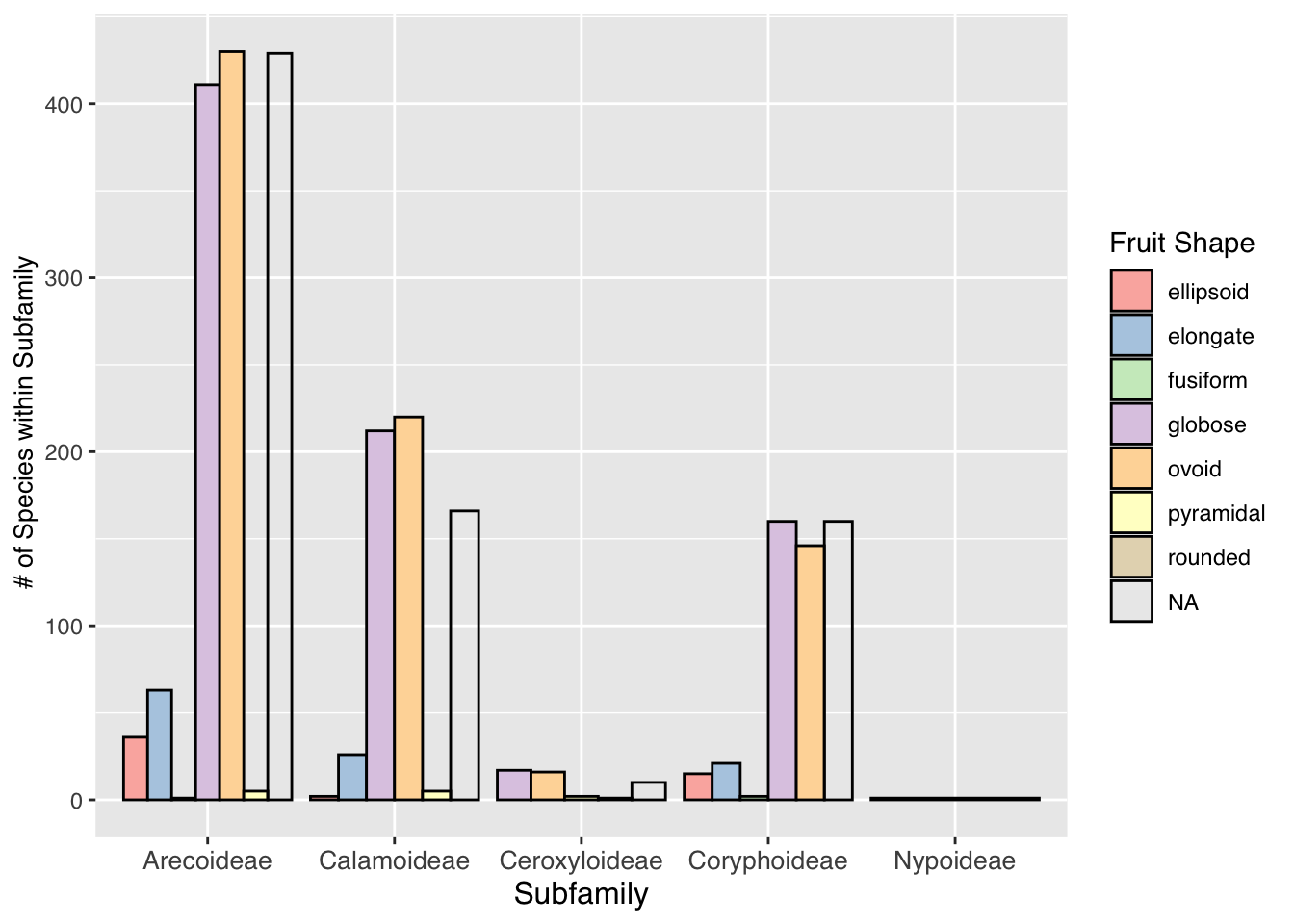
Pie chart:
- In this pie chart, I am looking at the
frequency of each palm tree subfamilies within the data set. It shows
that the subfamily, Arecoideae, is most common.
palm_piechart <- ggpie::ggpie(data=palmtrees,
                             group_key="palm_subfamily",
                             count_type="full",
                             label_info="ratio",
                             label_type="none") +
                            scale_fill_brewer(palette = "Pastel1") +
                            labs(fill = "Subfamily Name") +
                            theme(text = element_text(family = "Helvetica"))

palm_piechart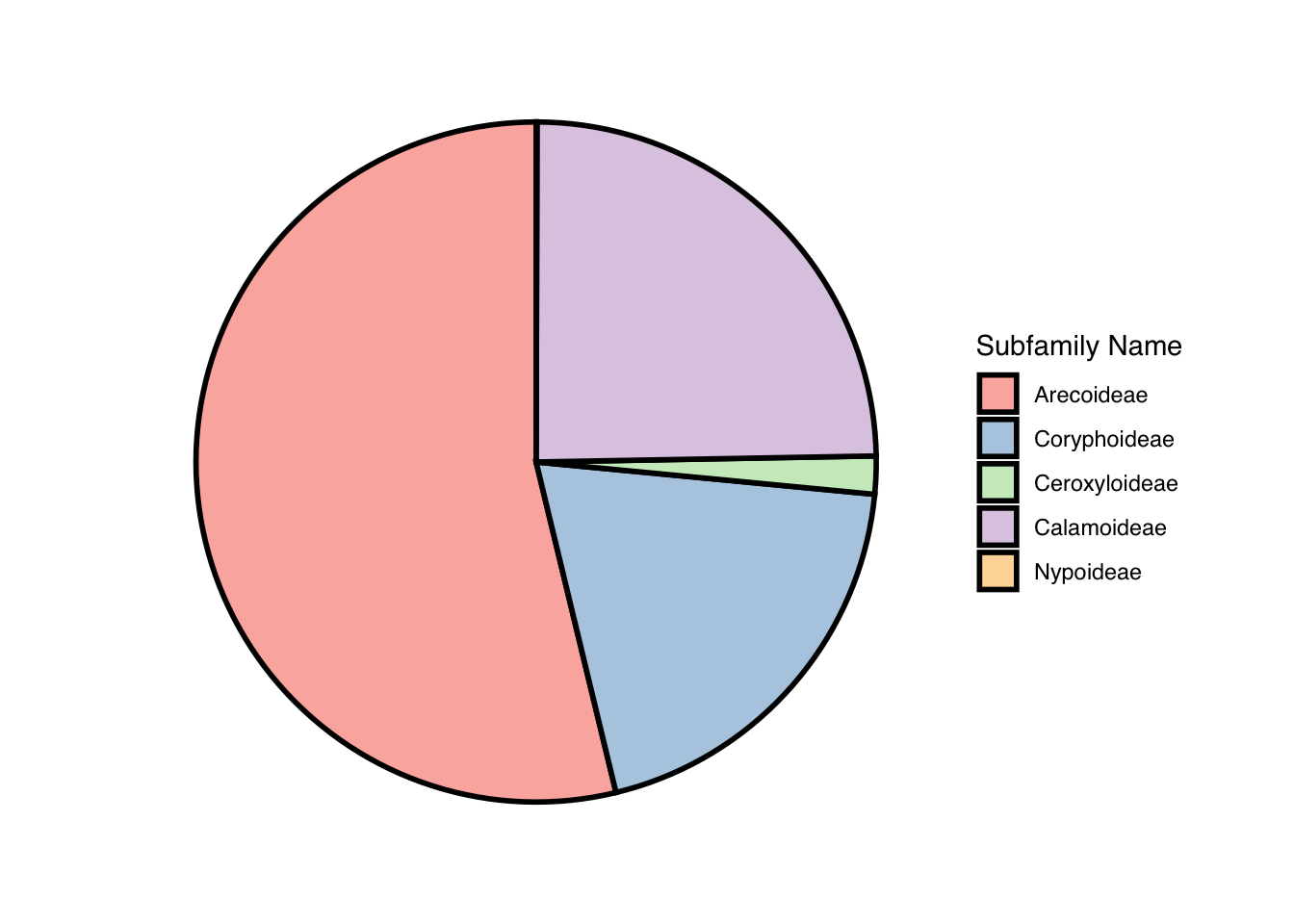
For the remaining figures, I subset the data set by subfamily using the following code:
arecoideae <- palmtrees[which(palmtrees$palm_subfamily == "Arecoideae"),]
calamoideae <- palmtrees[which(palmtrees$palm_subfamily == "Calamoideae"),]
ceroxyloideae <- palmtrees[which(palmtrees$palm_subfamily == "Ceroxyloideae"),]
coryphoideae <- palmtrees[which(palmtrees$palm_subfamily == "Coryphoideae"),]
nypoideae <- palmtrees[which(palmtrees$palm_subfamily == "Nypoideae"),]
Beeswarm Plot:
- Using a beeswarm plot, I wanted to see if
there is a relationship between palm trees in the subfamily,
Calamoideae, and whether species within that subfamily exhibit
“climbing” behavior (climb, don’t climb, or do both) in relation to
their maximum petiole length. It shows that species that climb have a
longer petiole length compared to non-climbers and palm trees in both
categories.
palm_beeswarm <- ggplot(data=calamoideae) +
                            aes(x=climbing,y=max__petiole_length_m,color=climbing) +
                            ggbeeswarm::geom_beeswarm(method = "center",size=3) +
                            scale_color_brewer(palette = "Accent") +
                            labs(x = "Climbing Type", y = "Maximum Petiole Length") +
                            theme(legend.position="none") +
                            theme(text = element_text(family = "Helvetica"),
                                  axis.title.x = element_text(size = 12),
                                  axis.text.x = element_text(size = 10),
                                  axis.title.y = element_text(size = 12))

palm_beeswarm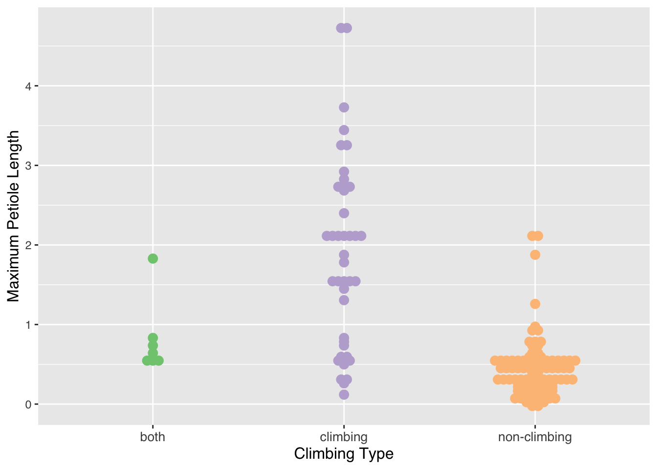
Waffle plot:
- Using a waffle plot, I wanted to see how
many tribes are within the subfamily, Coryphoideae. This waffle plot
shows the number of species within each tribe.
tabled_data <- as.data.frame(table(class=coryphoideae$palm_tribe))

palm_waffle <- ggplot(data=tabled_data) +
                          aes(fill = class, values = Freq) +
                          waffle::geom_waffle(n_rows = 10, size = 0.3, colour = "white") +
                          scale_fill_manual(name = "Tribe Names:",
                                            values = c("#698B69", "#528B8B","#CD8C95", "#B2DFEE", "#EE9572","#CDCDC1","#CD96CD","#CDBA96"),
                                            labels = c("Borasseae", "Caryoteae", "Chuniophoeniceae","Corypheae","Cryosophileae","Phoeniceae","Sabaleae","Trachycarpeae")) +
                          coord_equal() +
                          theme_void() +
                          theme(legend.position = "bottom", text = element_text(family = "Helvetica"))

palm_waffle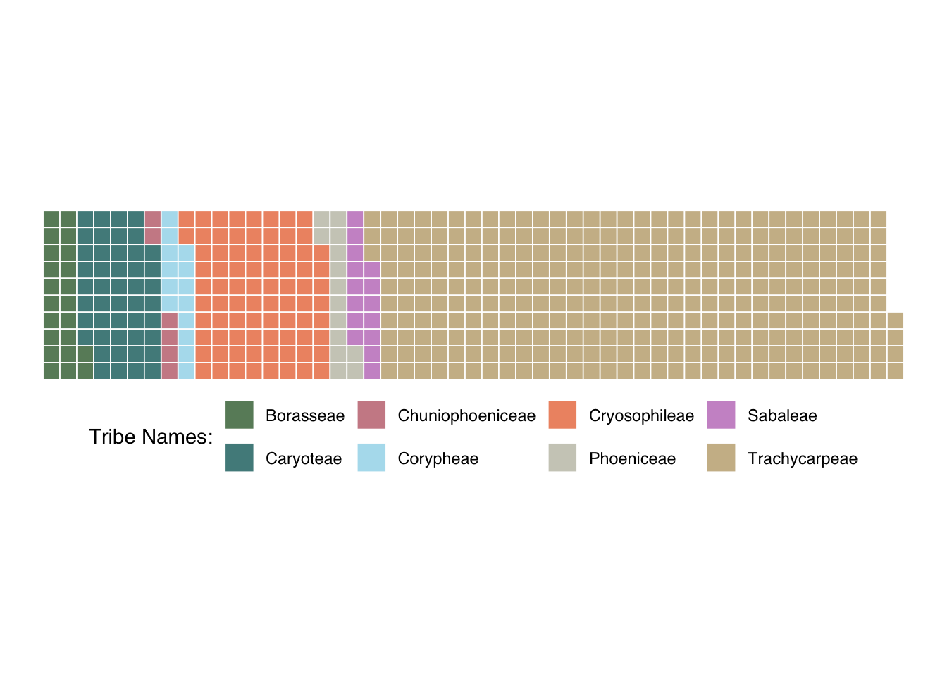
Ridgeline plot:
- This ridgeline plot shows the
distribution of maximum stem height (m) by subfamily.
palm_subfamily_df <- data.frame(palmtrees$palm_subfamily)
palm_stemheight_df <- data.frame(palmtrees$max_stem_height_m)
palm_df <- cbind(palm_subfamily_df, palm_stemheight_df)
palm_df_clean <- palm_df[complete.cases(palm_df),]

palm_ridgeline <- ggplot(data=palm_df_clean,
                         aes(x=palmtrees.max_stem_height_m,y=palmtrees.palm_subfamily, fill = palmtrees.palm_subfamily)) +
                         scale_fill_brewer(palette = "Accent") +
                         ggridges::geom_density_ridges(scale = 0.9) +
                         ggridges::theme_ridges() +
                         scale_x_continuous(limits = c(-10,100)) +
                         xlab("Maximum stem height (m)") +
                         ylab("Subfamily") +
                         theme(legend.position = "none", text = element_text(family = "Helvetica"))

palm_ridgeline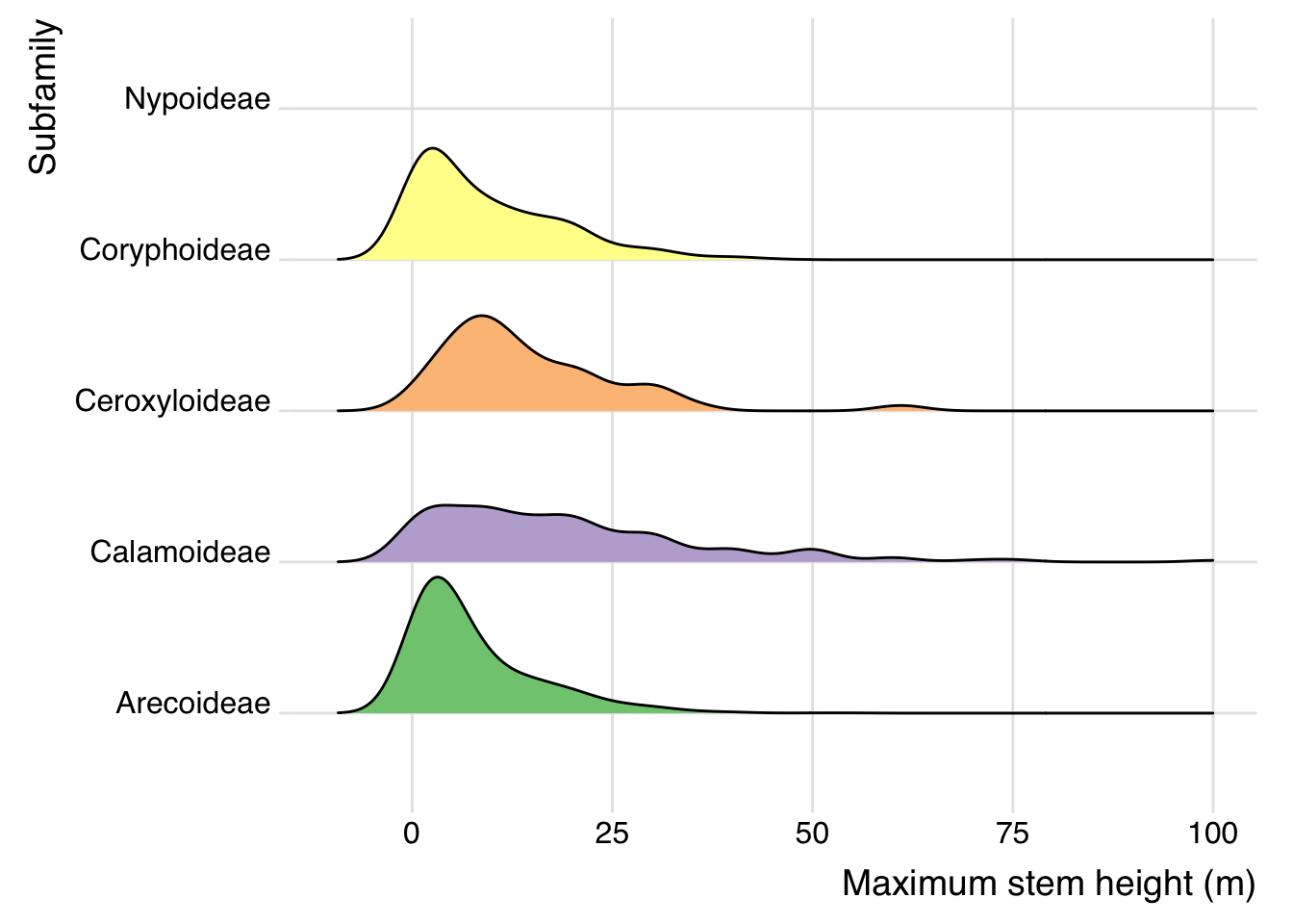
Saving each plots:
ggsave(palm_piechart,file="palm_piechart.png",width=10,height=6,bg = "white")
ggsave(palm_beeswarm,file="palm_beeswarm.png",width=10,height=6,bg = "white")
ggsave(palm_waffle,file="palm_waffle.png",width=10,height=6,bg = "white")
ggsave(palm_ridgeline,file="palm_ridgeline.png",width=10,height=6,bg = "white")